Refer to the 2005 example (document) also.
Break the Knudsen chirp processing into two steps because
SIOSEIS process GAINS needs to be used twice.
Script to make envelopes.
Script to make a sioseis plot from envelopes.
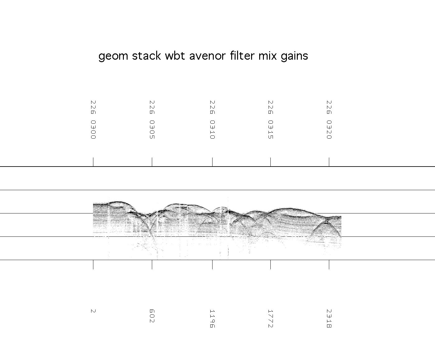
Plot - procs diskin prout geom stack wbt avenor filter mix gains plot end
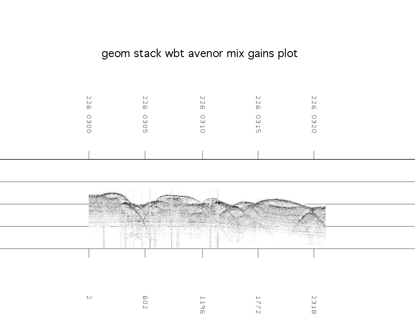
Plot - procs diskin prout geom stack wbt avenor mix gains plot end
Plot - procs diskin prout geom stack wbt avenor filter gains plot end
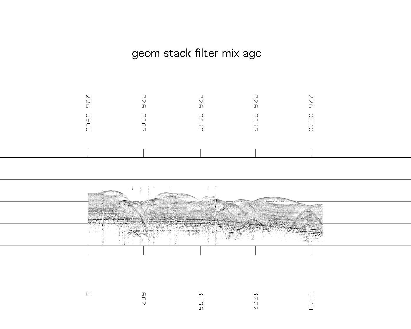
Plot - procs diskin prout geom stack wbt filter mix agc plot end
Plot - procs diskin prout geom stack wbt agc filter mix plot end
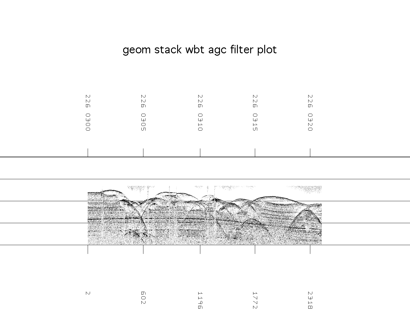
Plot - procs diskin prout geom stack wbt agc filter plot end
Swath map
Comments on Script 1:
1) Process header is used to save the number of samples in trace in a different
word in the SEG-Y trace header because the FFTs in T2F will expand the trace
to the next larger power of two. Sort integer word 58 contains the number of
samples, so i120 = i58 means save the contents of header word 58 in word 120.
e.g. If there are 11111 samples, the next larger power of two is 16384.
Without using the header scheme, the output would be 16384 samples.
2) t2f creates the analytic signal and then gains does the complex modulus to
create the envelope.
3) The SEG-Y standard uses a 16bit integer for the number of samples. SIOSEIS
uses a 16 bit unsigned integer under the rationalization that the number of
samples can not be negative. t2f creates complex numbers, so it creates twice
the number of samples. The Knudsen often creates traces with 22222 sample,
which means the fft makes it 32768 complex samples or 65536 words, which sioseis
can deal with.
Comments on Script 2:
1) Process GEOM type 17 computes the distance along the ship track line of every
trace. DBRPS 3 uses a 3m bin spacing so that traces within 3 meters will be
flagged as being in the same position.o that process stack can sum them.
Process GEOM also sets the distance from the first trace of the job into the
SEG-Y header "range" location.
2) There are two distinct processing sequences described. The first set
assumes the water bottom depth picked by Knudsen is valid most of the time.
Process wbt converts depth to time and save the time in SEG-Y header word
50, which other processes such as gains recognizes. When a zero depth is
encountered, which Knudsen uses to indicate no pick, WBT uses the last good
depth.
The second set of examples does not require water depths.
3) Both sets of examples use some type of trace equalization. Trace
equalization is needed becuase the trace to trace amplitudes vary when
the Knudsen pulse length changes or when the transducer transmit or
receive power is changed. The avenor method equalizes the traces based
on the average amplitude within .1 seconds of the Knudsen picked water
bottom. The other method uses AGC which equalizes in time and space.
4) The plots don't show much difference with a two trace running mix, but
remember that random noise is cancelled by the square root of the number
of things added. SQRT(2) helps and a two trace mix is fine with deep dip.
5) The gain used in process gains is e**(5*t), hung from the water bottom
(t0 = water bottom).
Comments about plotting by range
The Knudsen does not "fire by distance", rather it's ping rate is determined
by the water depth. They don't want multiple pings in the water simultaneously,
so the ping rate is high in shallow water and low in deep water.
Another source of ship speed variation is the varying ice conditions.
The Knudsen SEG-Y files contain a ship position, but which navigation system
is used is not known. It is also unknown how ping rates greater than 1 per
second obtain GPS fixes. Some fixes (lat/long) are the same as adjacent ones
even though the ship has moved (some GPS units do not report fixes more
frequently than 1 per second).
Determining the processing sequence
Plot of raw data, without ANY processing (every ping, no amplitude adjustments).
List of fixes for pings 29001-29050.
Plot AGC, winlen .025 center .001
Plot AVENOR (trace equalization based on water bottom)
Plot procs diskin prout wbt avenor filter(2x500) plot end
Plot procs diskin prout wbt avenor filter gains ( subwb yes type 5 alpha 20) plot end
Plot procs diskin prout wbt avenor filter mix (1 1) gains plot end
Plot procs diskin prout geom wbt avenor filter mix gains plot (hscale 300) end
hscale 300 was chosen because the plot resolution is 300 dots per inch,
thus the distance between the tyraces on the plot will be 1 meter. The
spaces in the plot are because the distance between traces is greater
than 1 (see the above list). e.g. if the distance between traces is 1.1
meters, then there are only 9 traces for every 10 lines on the plot.
Plot procs diskin prout geom stack (1m bin) wbt avenor filter mix gains plot
"Sorting" or binning the data into 1m bins (binning is a multi-channel
seismic technique) and then stacking results in many more gaps in the plot.
Some bins have multiple traces that are summed and some bins are empty,
again, because the average distance between pings is 1.1m
Plot procs diskin prout geom stack (3m bin) wbt avenor filter mix gains (alpha 5) plot (hscale 900)
Three meter stack bins with plot spacing of 900m/inch still results
in some spaces.
Plot procs diskin prout geom stack wbt avenor filter mix gains plot end
Conclusion
Three meter stack bins without plotting by range is the best for HLY0602
when the ship is plodding along at 2-3 kts. in water depths < 1500m and
the Knudsen with a 12ms pulse (think rep rate).
Using this geom/stack method eliminates the display problems when the
ship is stopped (for coring) or backing-and-ramming.
Back to SIOSEIS Examples.
Go to the list of seismic processes.
Go to SIOSEIS introduction.